Mixture of two normals • mastiff

Consider the following model:

$i$ indexes the observation
The unobserved binary variable $d_i$ equals 1 with probability $p_i$ , 0 otherwise: $d_i \: | \: p_i \sim \text{Bernoulli}(p_i)$
The observed variable $y_i$ is normally distributed with parameters $\mu_0, \sigma_0$ if $d_i=0$ , or normally distributed with parameters $\mu_1, \sigma_1$ if $d_i=1$ . We can write this in a single equation: $P(y_i \: | \: d_i, \mu_1, \sigma_1, \mu_0, \sigma_0) = d_i N(y_i \: | \: \mu_1, \sigma_1) + (1-d_i) N(y_i \: | \: \mu_0, \sigma_0)$ For identifiability we define $\mu_0 \leq \mu_1$ , i.e. whichever normal has the smaller mean we define to be $d=0$ . We obtain the unconditional probability of $y_i$ without knowing $d_i$ by marginalising over $d_i$ , giving a mixture of the two normals: $\begin{aligned} P(y_i \: | \: p_i, \mu_1, \sigma_1, \mu_0, \sigma_0) = & \sum_{d_i} P(y_i \: | \: d_i, \mu_1, \sigma_1, \mu_0, \sigma_0) P(d_i \: | \: p_i) \\ = & p_i N(y_i \: | \: \mu_1, \sigma_1) + (1-p_i) N(y_i \: | \: \mu_0, \sigma_0)\end{aligned}$
There are $n$ discrete groups, indexed by $g \in [1, 2, \ldots n]$ , which differ in their probabilities for $d$ : $p_g$ is the probability that $d_i=1$ if $i$ is in $g$ . Parameterise the variability between $p_g$ values with an overall parameter $p$ , a length- $n$ vector $\boldsymbol{\beta}$ of unconstrained regression coefficients, and a logit link function to keep probability parameters between 0 and 1: $p_g = \text{logistic}(\text{logit}(p) + \beta_g)$ . We thus use $n+1$ parameters to describe $n$ degrees of freedom, but this allows us to have identical and correlated priors for the $n$ different groups (as opposed to picking one group as a reference and parameterising others relative to it, introducing greater uncertainty for the non-reference groups even before conditioning on the data). Specifically we model the different components of the vector $\boldsymbol{\beta}$ as normally distributed, independently given a scale parameter $\sigma^\text{groups}$ : $\beta_g \: | \: \sigma^\text{groups} \sim N(0, \sigma^\text{groups})$
The design matrix $x_{ig}$ , which is observed, equals 1 if observation $i$ is in group $g$ , 0 otherwise. So $p_i = \sum_g x_{ig} p_g = \text{logistic}(\text{logit}(p) + \sum_g x_{ig} \beta_g)$ .

In summary, we have a logistic random-effects regression model for $d$ , and two-component normal mixture model for $y$ with $d$ indicating which component.

Set up our session

suppressPackageStartupMessages(library(mastiff))
suppressPackageStartupMessages(library(dplyr))
suppressPackageStartupMessages(library(ggplot2))
suppressPackageStartupMessages(library(magrittr))
suppressPackageStartupMessages(library(tidyr))
suppressPackageStartupMessages(library(stringr))

theme_set(theme_classic())
set.seed(12345) # For reproducibility

Simulate some data from a mixture of two normal distributions:

groups <- LETTERS[1:5]
results <- simulate_mixture_of_two_normals(n = 500,
                                           groups = groups,
                                           sd_groups = 2)
df_data <- results$data
params <- results$params

Inspect the data

head(df_data)
#>   group     d          y
#> 1     B  TRUE  3.8892457
#> 2     C FALSE  0.5479883
#> 3     B  TRUE  2.1813534
#> 4     A  TRUE  1.7631771
#> 5     A  TRUE  5.3172256
#> 6     D FALSE -0.1556485

Plot all the data

ggplot(df_data) +
  geom_histogram(aes(y), bins = 30) +
  coord_cartesian(expand = FALSE)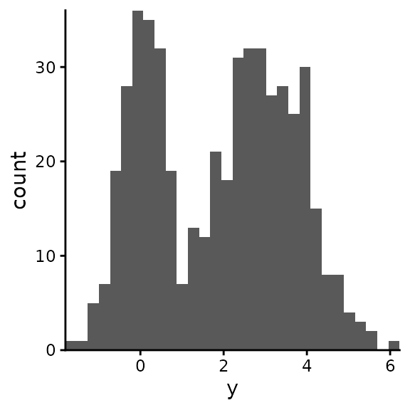

Visualise the two normals separately:

ggplot(df_data) +
  geom_histogram(aes(y, fill = as.factor(as.integer(d))),
                 position = "identity",
                 alpha = 0.6,
                 bins = 30) +
  coord_cartesian(expand = FALSE) +
  labs(fill = "d")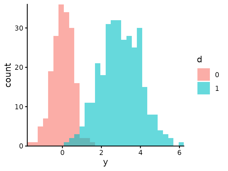

Estimate the parameters using Bayesian inference. For almost all parameters we use uniform priors with specified upper and lower bounds. (‘Almost all’ means all except the normally varying components of $\boldsymbol\beta$ , the group-specific values of $p$ that are defined by $\boldsymbol\beta$ , and $\mu_1$ for which we specify a minimum and maximum but it is constrained to be greater than $\mu_0$ .)

prior_boundaries <- tribble(
  ~param, ~lower, ~upper,
  "mu_0", -10, 10,
  "mu_1", -10, 10,
  "sd_0", 0, 5,
  "sd_1", 0, 5,
  "sd_groups", 0, 3,
  "p", 0, 1
  )
df_samples_posterior <- estimate_mixture_of_two_normals(
  y = df_data$y,
  groups = df_data$group, 
  prior_boundaries = prior_boundaries,
  report_stan_progress = TRUE)
#> 
#> SAMPLING FOR MODEL 'mixture_of_two_normals' NOW (CHAIN 1).
#> Chain 1: 
#> Chain 1: Gradient evaluation took 0.00023 seconds
#> Chain 1: 1000 transitions using 10 leapfrog steps per transition would take 2.3 seconds.
#> Chain 1: Adjust your expectations accordingly!
#> Chain 1: 
#> Chain 1: 
#> Chain 1: Iteration:    1 / 2000 [  0%]  (Warmup)
#> Chain 1: Iteration:  200 / 2000 [ 10%]  (Warmup)
#> Chain 1: Iteration:  400 / 2000 [ 20%]  (Warmup)
#> Chain 1: Iteration:  600 / 2000 [ 30%]  (Warmup)
#> Chain 1: Iteration:  800 / 2000 [ 40%]  (Warmup)
#> Chain 1: Iteration: 1000 / 2000 [ 50%]  (Warmup)
#> Chain 1: Iteration: 1001 / 2000 [ 50%]  (Sampling)
#> Chain 1: Iteration: 1200 / 2000 [ 60%]  (Sampling)
#> Chain 1: Iteration: 1400 / 2000 [ 70%]  (Sampling)
#> Chain 1: Iteration: 1600 / 2000 [ 80%]  (Sampling)
#> Chain 1: Iteration: 1800 / 2000 [ 90%]  (Sampling)
#> Chain 1: Iteration: 2000 / 2000 [100%]  (Sampling)
#> Chain 1: 
#> Chain 1:  Elapsed Time: 5.979 seconds (Warm-up)
#> Chain 1:                4.353 seconds (Sampling)
#> Chain 1:                10.332 seconds (Total)
#> Chain 1: 
#> 
#> SAMPLING FOR MODEL 'mixture_of_two_normals' NOW (CHAIN 2).
#> Chain 2: 
#> Chain 2: Gradient evaluation took 0.000143 seconds
#> Chain 2: 1000 transitions using 10 leapfrog steps per transition would take 1.43 seconds.
#> Chain 2: Adjust your expectations accordingly!
#> Chain 2: 
#> Chain 2: 
#> Chain 2: Iteration:    1 / 2000 [  0%]  (Warmup)
#> Chain 2: Iteration:  200 / 2000 [ 10%]  (Warmup)
#> Chain 2: Iteration:  400 / 2000 [ 20%]  (Warmup)
#> Chain 2: Iteration:  600 / 2000 [ 30%]  (Warmup)
#> Chain 2: Iteration:  800 / 2000 [ 40%]  (Warmup)
#> Chain 2: Iteration: 1000 / 2000 [ 50%]  (Warmup)
#> Chain 2: Iteration: 1001 / 2000 [ 50%]  (Sampling)
#> Chain 2: Iteration: 1200 / 2000 [ 60%]  (Sampling)
#> Chain 2: Iteration: 1400 / 2000 [ 70%]  (Sampling)
#> Chain 2: Iteration: 1600 / 2000 [ 80%]  (Sampling)
#> Chain 2: Iteration: 1800 / 2000 [ 90%]  (Sampling)
#> Chain 2: Iteration: 2000 / 2000 [100%]  (Sampling)
#> Chain 2: 
#> Chain 2:  Elapsed Time: 5.725 seconds (Warm-up)
#> Chain 2:                4.337 seconds (Sampling)
#> Chain 2:                10.062 seconds (Total)
#> Chain 2: 
#> 
#> SAMPLING FOR MODEL 'mixture_of_two_normals' NOW (CHAIN 3).
#> Chain 3: 
#> Chain 3: Gradient evaluation took 0.000141 seconds
#> Chain 3: 1000 transitions using 10 leapfrog steps per transition would take 1.41 seconds.
#> Chain 3: Adjust your expectations accordingly!
#> Chain 3: 
#> Chain 3: 
#> Chain 3: Iteration:    1 / 2000 [  0%]  (Warmup)
#> Chain 3: Iteration:  200 / 2000 [ 10%]  (Warmup)
#> Chain 3: Iteration:  400 / 2000 [ 20%]  (Warmup)
#> Chain 3: Iteration:  600 / 2000 [ 30%]  (Warmup)
#> Chain 3: Iteration:  800 / 2000 [ 40%]  (Warmup)
#> Chain 3: Iteration: 1000 / 2000 [ 50%]  (Warmup)
#> Chain 3: Iteration: 1001 / 2000 [ 50%]  (Sampling)
#> Chain 3: Iteration: 1200 / 2000 [ 60%]  (Sampling)
#> Chain 3: Iteration: 1400 / 2000 [ 70%]  (Sampling)
#> Chain 3: Iteration: 1600 / 2000 [ 80%]  (Sampling)
#> Chain 3: Iteration: 1800 / 2000 [ 90%]  (Sampling)
#> Chain 3: Iteration: 2000 / 2000 [100%]  (Sampling)
#> Chain 3: 
#> Chain 3:  Elapsed Time: 5.959 seconds (Warm-up)
#> Chain 3:                4.044 seconds (Sampling)
#> Chain 3:                10.003 seconds (Total)
#> Chain 3: 
#> 
#> SAMPLING FOR MODEL 'mixture_of_two_normals' NOW (CHAIN 4).
#> Chain 4: 
#> Chain 4: Gradient evaluation took 0.000157 seconds
#> Chain 4: 1000 transitions using 10 leapfrog steps per transition would take 1.57 seconds.
#> Chain 4: Adjust your expectations accordingly!
#> Chain 4: 
#> Chain 4: 
#> Chain 4: Iteration:    1 / 2000 [  0%]  (Warmup)
#> Chain 4: Iteration:  200 / 2000 [ 10%]  (Warmup)
#> Chain 4: Iteration:  400 / 2000 [ 20%]  (Warmup)
#> Chain 4: Iteration:  600 / 2000 [ 30%]  (Warmup)
#> Chain 4: Iteration:  800 / 2000 [ 40%]  (Warmup)
#> Chain 4: Iteration: 1000 / 2000 [ 50%]  (Warmup)
#> Chain 4: Iteration: 1001 / 2000 [ 50%]  (Sampling)
#> Chain 4: Iteration: 1200 / 2000 [ 60%]  (Sampling)
#> Chain 4: Iteration: 1400 / 2000 [ 70%]  (Sampling)
#> Chain 4: Iteration: 1600 / 2000 [ 80%]  (Sampling)
#> Chain 4: Iteration: 1800 / 2000 [ 90%]  (Sampling)
#> Chain 4: Iteration: 2000 / 2000 [100%]  (Sampling)
#> Chain 4: 
#> Chain 4:  Elapsed Time: 6 seconds (Warm-up)
#> Chain 4:                4.232 seconds (Sampling)
#> Chain 4:                10.232 seconds (Total)
#> Chain 4:

For plotting purposes we sample from the prior as well as the posterior:

df_samples_prior <- estimate_mixture_of_two_normals(
  y = df_data$y,
  groups = df_data$group, 
  prior_boundaries = prior_boundaries,
  sample_posterior_not_prior = FALSE)

In a single plot, for each parameter, we compare the posterior to the prior and the posterior to the true value. (This is, respectively, to show the relative contributions of prior assumptions and data to our conclusions, and as a check that the statistical model was correctly implemented. Read more about doing this, and why you should always do it, in the vignette Plotting Stan output). Here we need the skip_stanfit_to_dt argument of plot_posterior() because we’re giving it samples stored as datatables instead of as stanfit objects. In the plot, each panel is one parameter, and the black vertical line is the true value.

plot_posterior(df_samples_posterior,
               prior_samples = df_samples_prior,
               true_param_values = params,
               skip_stanfit_to_dt = TRUE,
               params_desired = c("mu_0", "mu_1", "sd_0", "sd_1", "sd_groups", paste0("p_for_", groups)))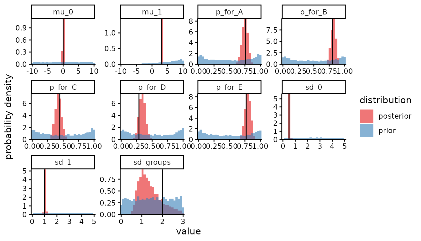

The estimation of sd_groups isn’t great, but that doesn’t matter provided our estimates of p for each group are OK. Next we investigate the distribution of $y$ after having marginalised over $d$ , i.e. the mixture of two normals, and how this distribution varies between groups. First we calculate the true distribution given the true parameters. For later convenience, at the same time as calculating $P(y) = P(y \: | \: d = 0) P(d = 0) + P(y \: | \: d = 1) P(d = 1)$ , we also calculate as a function of y $P(d = 1 \: | \: y) = P(y \: | \: d = 1) P(d = 1) / P(y)$ .

y_values <- seq(from = min(df_data$y) - 2, to = max(df_data$y) + 2, length.out = 100)
true_ps <- params[paste0("p_for_", groups)]
df_y_distributions_true <- tibble(p = true_ps,
                                  group = names(true_ps)) %>%
  mutate(group = str_remove(group, "p_for_")) %>%
  cross_join(tibble(y = y_values)) %>%
  mutate(`P(y | d = 1)` = dnorm(y, params[["mu_1"]], params[["sd_1"]]),
         `P(y | d = 0)` = dnorm(y, params[["mu_0"]], params[["sd_0"]]),
         `P(y)` = p * `P(y | d = 1)` + (1 - p) * `P(y | d = 0)`,
         `P(d = 1 | y)` = p * `P(y | d = 1)` / `P(y)`) %>%
  select(group, y, "P(y)", "P(d = 1 | y)") %>%
  pivot_longer(cols = c("P(y)", "P(d = 1 | y)"),
               names_to = "which_function_of_y")

Second we calculate the estimated distributions.

df_y_distributions <- df_samples_posterior %>%
  as_tibble() %>%
  mutate(sample = row_number()) %>%
  select("sample", "mu_0", "mu_1", "sd_0", "sd_1", paste0("p_for_", groups)) %>%
  pivot_longer(cols = paste0("p_for_", groups),
               names_to = "group",
               values_to = "p",
               names_prefix = "p_for_") %>%
  cross_join(tibble(y = y_values)) %>%
  mutate(`P(y | d = 1)` = dnorm(y, mu_1, sd_1),
         `P(y | d = 0)` = dnorm(y, mu_0, sd_0),
         `P(y)` = p * `P(y | d = 1)` + (1 - p) * `P(y | d = 0)`,
         `P(d = 1 | y)` = p * `P(y | d = 1)` / `P(y)`) %>%
  select("sample", "group", "y", "P(y)", "P(d = 1 | y)") %>%
  pivot_longer(cols = c("P(y)", "P(d = 1 | y)"),
               names_to = "which_function_of_y")

We plot both of these together with the data.

posterior_thinning_factor <- 10 # Keep one in every 10 samples
ggplot() +
  geom_histogram(data = df_data, aes(x = y, y = after_stat(density)),
                 bins = 30) +
  geom_line(data = df_y_distributions %>%
              filter(which_function_of_y == "P(y)",
                     sample %% posterior_thinning_factor == 0),
            aes(x = y, y = value, group = sample), alpha = 0.15) +
  geom_line(data = df_y_distributions_true %>%
              filter(which_function_of_y == "P(y)"),
            aes(x = y, y = value), col = "blue") +
  coord_cartesian(expand = FALSE) +
  facet_wrap(~group) +
  theme_classic() +
  labs(subtitle = paste0("Histogram = data.\nBlue line = true distribution.\n",
                         "Black lines = posterior samples for the estimated ",
                         "distribution.\nPosterior thinned by a factor ",
                         posterior_thinning_factor, " for visibility.")) +
  xlim(min(df_data$y), max(df_data$y))
#> Warning: Removed 10 rows containing missing values or values outside the scale range
#> (`geom_bar()`).
#> Warning: Removed 68000 rows containing missing values or values outside the scale range
#> (`geom_line()`).
#> Warning: Removed 170 rows containing missing values or values outside the scale range
#> (`geom_line()`).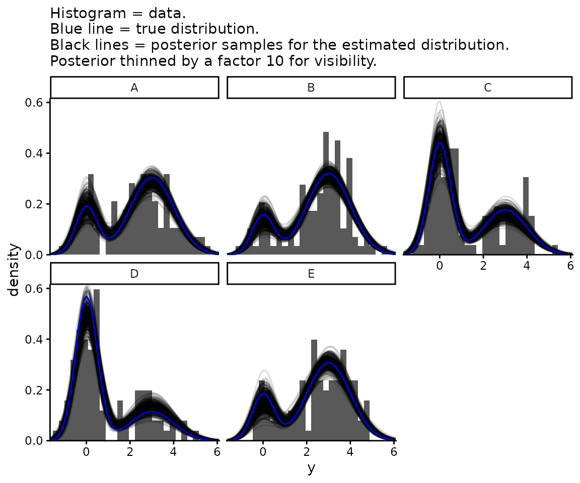

Now plot $P(d = 1 \: | \: y) = P(y \: | \: d = 1) P(d = 1) / P(y)$ , i.e. how likely each $y$ value is to have come from one normal distribution or the other.

ggplot() +
  geom_line(data = df_y_distributions %>%
              filter(which_function_of_y == "P(d = 1 | y)",
                     sample %% posterior_thinning_factor == 0),
            aes(x = y, y = value, group = sample), alpha = 0.15) +
  geom_line(data = df_y_distributions_true %>%
              filter(which_function_of_y == "P(d = 1 | y)"),
            aes(x = y, y = value), col = "blue") +
  coord_cartesian(expand = FALSE) +
  facet_wrap(~group) +
  theme_classic() +
  labs(subtitle = paste0("Blue line = true function.\n",
                         "Black lines = posterior samples for the estimated ",
                         "function.\nPosterior thinned by a factor ",
                         posterior_thinning_factor, " for visibility."))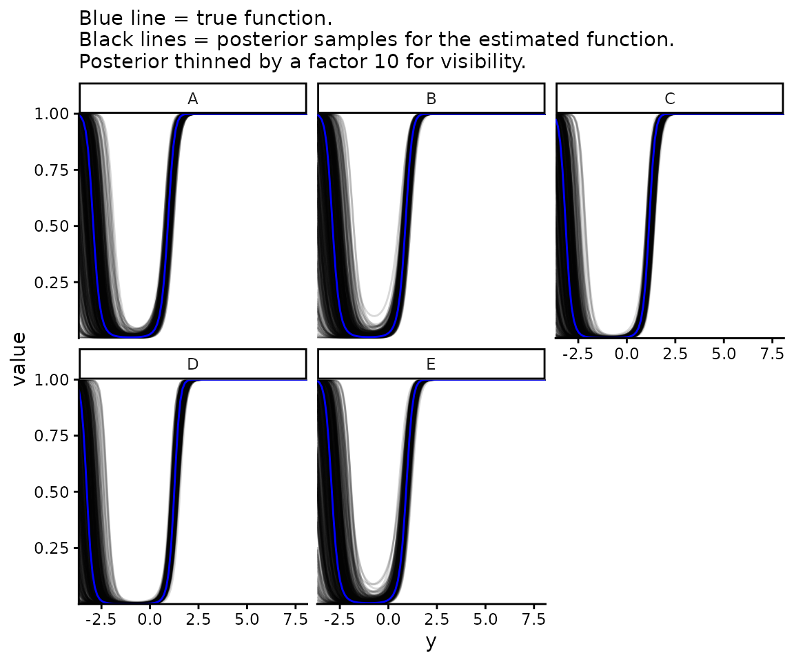

You can see at the smallest $y$ values that $P(d = 1 \: | \: y)$ is not monotonic in $y$ . This is always true for a mixture of two normal distributions unless they have identical variances. If they don’t, the one with the larger variances makes up an ever increasing proportion of the mixture at both asymptotically positive and asymptotically negative values of $y$ . This may be problematic for applications where we want $P(d = 1 \: | \: y)$ to be monotonic, i.e. where we believe that the larger $y$ is the more likely it is to come from $d=1$ (or from $d=0$ depending). In this case, the model may be an acceptable application if the fitted model is monotonic over the range of $y$ values of interest. If not, a different mixture model using a distribution other than a normal should be used.