Estimation on simulated data

Recap

dvsb estimates disease variability in subpopulations from biomarkers, e.g. estimating the variability between subpopulations in seroprevalence (the proportion of people who are seropositive) with antibody levels estimated using an assay measuring some proxy such as ELISA Optical Density values. We call the biomarker x (e.g. antibody level) and the proxy measurement y (e.g. OD values).

Setting up

library(dvsb)
library(tidyr)
library(dplyr)
library(ggplot2)
theme_set(theme_classic())

Let’s start by getting out of the way two clunky things. First, dvsb does not include pre-compiled binary (executable) files for the Stan models. This is for our (developer) convenience at the cost of your (user) inconvenience; it also means we can switch seamlessly between rstan, cmdstanr and cmdstan when interfacing to stan. The first time you call dvsb::run_stan_interfaces() after each installation or update of dvsb, the Stan code gets compiled into binary form. That happens automatically, but you do need to tell it where the Stan code lives after dvsb has been installed onto your system. Let’s find where that is:

stan_dir <- system.file("stan", package = "dvsb")
list.files(stan_dir, pattern = "*.stan")
#> [1] "dvsb_accidental_blanks.stan"  "dvsb_no_mu_x_predictors.stan"
#> [3] "dvsb.stan"

In that directory,

• dvsb.stan is the main dvsb model.
  
• dvsb_accidental_blanks.stan is the extended model that allows for the possibility that each sample well accidentally contains nothing at all (i.e. is blank).
  
• dvsb_no_mu_x_predictors.stan is the restricted model in which regression models are not specified for the means of the two antibody distributions (one for seropositives and one for seronegatives).

Let’s use the main model.

stan_path <- file.path(stan_dir, "dvsb.stan")

The second clunky thing: a dataframe’s worth of input specifying the priors is required. We store this in a csv file bundled with dvsb, so that you can more easily inspect it, modify it, make different copies for different analyses, move copies outside of your dvsb repository in case prior defaults are updated in later changes to dvsb, etc. Again, you just need to say where this file lives after dvsb has been installed on your system. We find where that is similarly:

priors_dir <- system.file("input_priors", package = "dvsb")
list.files(priors_dir)
#> [1] "priors.csv"

Now set the path to that file - the one bundled with dvsb. (If you want to use a copy of this file that you moved somewhere else and perhaps modified, you would give that path instead.)

priors_path <- file.path(priors_dir, "priors.csv")

OK those clunky things are done. Phew. Read in the prior file, giving us a list with three things in it:

priors_list <- read_priors(priors_path)
df_priors_scalars <- priors_list$df_priors_scalars
df_priors_vectors <- priors_list$df_priors_vectors
rho_prior_eta <- priors_list$rho_prior_eta

Simulate data

Next we simulate data, giving us a list with seven things in it. (If we were using real data instead of simulated data, we would simply need to create the df_sam and df_cal dataframes ourselves instead of running simulate_data() below. The documentation for prepare_data_for_stan() explains what columns these dataframes require, and how sets of covariates for regression models are specified using the arguments x_mix_pred_vars_names, p_pos_binary_pred_vars, f_pred_vars_names.)

data <- simulate_data(seed = 1234,
                      num_sam_per_plate = 100)
df_sam <- data$df_sam
df_cal <- data$df_cal
df_plate <- data$df_plate
param_true_values_list <- data$params
f_pred_vars_names <- data$f_pred_vars_names
x_mix_pred_vars_names <- data$x_mix_pred_vars_names
p_pos_binary_pred_vars <- data$p_pos_binary_pred_vars

Plot the simulated calibration data (one facet per plate):

ggplot(df_cal) +
  geom_point(aes(x = x, y = y)) +
  facet_wrap(~plate, ncol = 2) +
  theme_classic()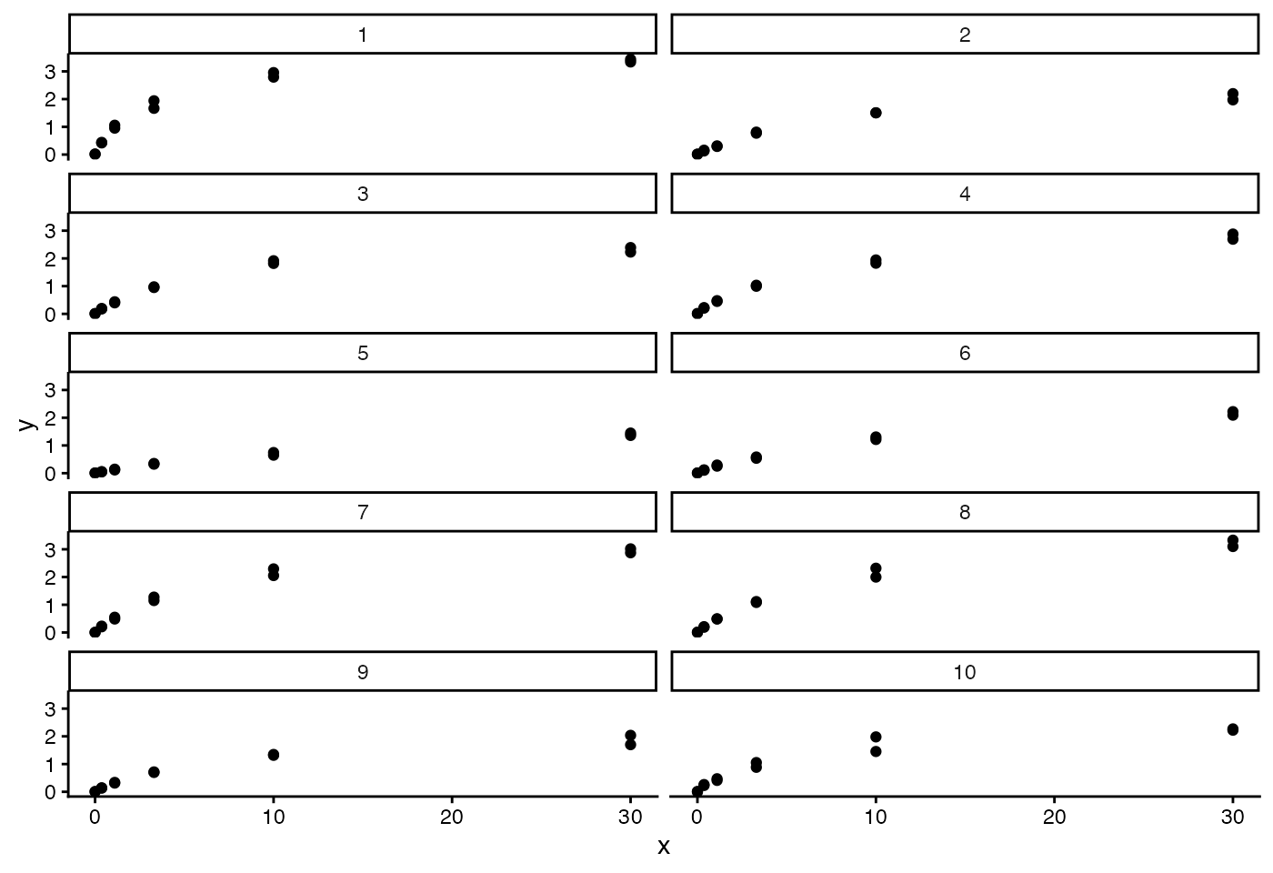

Plot the simulated sample data, histogramming the OD values, one facet for each category of the letter covariate (which differ in their x distributions when using default arguments for simulate_data()):

ggplot(df_sam) +
  geom_histogram(aes(x = x), bins = 20) +
  facet_wrap(~letter) +
  theme_classic() +
  scale_x_log10()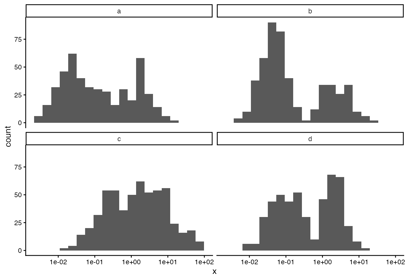

Run Stan

Wrangle the data and priors into the form needed for stan.

data_wrangled <- prepare_data_for_stan(
  df_sam = df_sam, 
  df_cal = df_cal, 
  df_priors_scalars = df_priors_scalars,
  df_priors_vectors = df_priors_vectors, 
  rho_prior_eta = rho_prior_eta, 
  x_mix_pred_vars_names = x_mix_pred_vars_names, 
  p_pos_binary_pred_vars = p_pos_binary_pred_vars,
  f_pred_vars_names = f_pred_vars_names
  )

Update our dataframes for samples, calibrators and plates with the extra columns we just added (which introduce integer indexing).

df_sam <- data_wrangled$df_sam
df_cal <- data_wrangled$df_cal
df_plate <- dplyr::left_join(df_plate, data_wrangled$df_plate, by = "plate") 

We specify some options controlling how Stan runs (see the help for run_stan_interfaces() for more information), then run Stan once to sample from the posterior, and again to sample from the prior¹.

df_posterior <- run_stan_interfaces(
  input_to_stan = data_wrangled$stan_input_posterior,
  path_to_stan_code = stan_path)
#> Started running Stan at[1] "2026-09-15 18:10:03 BST"
#> 
#> SAMPLING FOR MODEL 'anon_model' NOW (CHAIN 2).
#> 
#> SAMPLING FOR MODEL 'anon_model' NOW (CHAIN 1).
#> 
#> SAMPLING FOR MODEL 'anon_model' NOW (CHAIN 3).
#> 
#> SAMPLING FOR MODEL 'anon_model' NOW (CHAIN 4).
#> Chain 2: 
#> Chain 2: Gradient evaluation took 0.002679 seconds
#> Chain 2: 1000 transitions using 10 leapfrog steps per transition would take 26.79 seconds.
#> Chain 2: Adjust your expectations accordingly!
#> Chain 2: 
#> Chain 2: 
#> Chain 1: 
#> Chain 1: Gradient evaluation took 0.017264 seconds
#> Chain 1: 1000 transitions using 10 leapfrog steps per transition would take 172.64 seconds.
#> Chain 1: Adjust your expectations accordingly!
#> Chain 1: 
#> Chain 1: 
#> Chain 2: Iteration:   1 / 500 [  0%]  (Warmup)
#> Chain 3: 
#> Chain 3: Gradient evaluation took 0.003671 seconds
#> Chain 3: 1000 transitions using 10 leapfrog steps per transition would take 36.71 seconds.
#> Chain 3: Adjust your expectations accordingly!
#> Chain 3: 
#> Chain 3: 
#> Chain 3: Iteration:   1 / 500 [  0%]  (Warmup)
#> Chain 1: Iteration:   1 / 500 [  0%]  (Warmup)
#> Chain 4: 
#> Chain 4: Gradient evaluation took 0.002482 seconds
#> Chain 4: 1000 transitions using 10 leapfrog steps per transition would take 24.82 seconds.
#> Chain 4: Adjust your expectations accordingly!
#> Chain 4: 
#> Chain 4: 
#> Chain 4: Iteration:   1 / 500 [  0%]  (Warmup)
#> Chain 4: Iteration:  50 / 500 [ 10%]  (Warmup)
#> Chain 3: Iteration:  50 / 500 [ 10%]  (Warmup)
#> Chain 2: Iteration:  50 / 500 [ 10%]  (Warmup)
#> Chain 1: Iteration:  50 / 500 [ 10%]  (Warmup)
#> Chain 3: Iteration: 100 / 500 [ 20%]  (Warmup)
#> Chain 4: Iteration: 100 / 500 [ 20%]  (Warmup)
#> Chain 2: Iteration: 100 / 500 [ 20%]  (Warmup)
#> Chain 1: Iteration: 100 / 500 [ 20%]  (Warmup)
#> Chain 3: Iteration: 150 / 500 [ 30%]  (Warmup)
#> Chain 4: Iteration: 150 / 500 [ 30%]  (Warmup)
#> Chain 2: Iteration: 150 / 500 [ 30%]  (Warmup)
#> Chain 3: Iteration: 200 / 500 [ 40%]  (Warmup)
#> Chain 1: Iteration: 150 / 500 [ 30%]  (Warmup)
#> Chain 4: Iteration: 200 / 500 [ 40%]  (Warmup)
#> Chain 2: Iteration: 200 / 500 [ 40%]  (Warmup)
#> Chain 1: Iteration: 200 / 500 [ 40%]  (Warmup)
#> Chain 3: Iteration: 250 / 500 [ 50%]  (Warmup)
#> Chain 3: Iteration: 251 / 500 [ 50%]  (Sampling)
#> Chain 4: Iteration: 250 / 500 [ 50%]  (Warmup)
#> Chain 4: Iteration: 251 / 500 [ 50%]  (Sampling)
#> Chain 2: Iteration: 250 / 500 [ 50%]  (Warmup)
#> Chain 2: Iteration: 251 / 500 [ 50%]  (Sampling)
#> Chain 1: Iteration: 250 / 500 [ 50%]  (Warmup)
#> Chain 1: Iteration: 251 / 500 [ 50%]  (Sampling)
#> Chain 3: Iteration: 300 / 500 [ 60%]  (Sampling)
#> Chain 4: Iteration: 300 / 500 [ 60%]  (Sampling)
#> Chain 2: Iteration: 300 / 500 [ 60%]  (Sampling)
#> Chain 1: Iteration: 300 / 500 [ 60%]  (Sampling)
#> Chain 3: Iteration: 350 / 500 [ 70%]  (Sampling)
#> Chain 4: Iteration: 350 / 500 [ 70%]  (Sampling)
#> Chain 2: Iteration: 350 / 500 [ 70%]  (Sampling)
#> Chain 1: Iteration: 350 / 500 [ 70%]  (Sampling)
#> Chain 3: Iteration: 400 / 500 [ 80%]  (Sampling)
#> Chain 4: Iteration: 400 / 500 [ 80%]  (Sampling)
#> Chain 2: Iteration: 400 / 500 [ 80%]  (Sampling)
#> Chain 1: Iteration: 400 / 500 [ 80%]  (Sampling)
#> Chain 3: Iteration: 450 / 500 [ 90%]  (Sampling)
#> Chain 4: Iteration: 450 / 500 [ 90%]  (Sampling)
#> Chain 2: Iteration: 450 / 500 [ 90%]  (Sampling)
#> Chain 1: Iteration: 450 / 500 [ 90%]  (Sampling)
#> Chain 3: Iteration: 500 / 500 [100%]  (Sampling)
#> Chain 3: 
#> Chain 3:  Elapsed Time: 34.684 seconds (Warm-up)
#> Chain 3:                32.938 seconds (Sampling)
#> Chain 3:                67.622 seconds (Total)
#> Chain 3: 
#> Chain 4: Iteration: 500 / 500 [100%]  (Sampling)
#> Chain 4: 
#> Chain 4:  Elapsed Time: 38.487 seconds (Warm-up)
#> Chain 4:                32.772 seconds (Sampling)
#> Chain 4:                71.259 seconds (Total)
#> Chain 4: 
#> Chain 2: Iteration: 500 / 500 [100%]  (Sampling)
#> Chain 2: 
#> Chain 2:  Elapsed Time: 39.993 seconds (Warm-up)
#> Chain 2:                33.376 seconds (Sampling)
#> Chain 2:                73.369 seconds (Total)
#> Chain 2: 
#> Chain 1: Iteration: 500 / 500 [100%]  (Sampling)
#> Chain 1: 
#> Chain 1:  Elapsed Time: 40.69 seconds (Warm-up)
#> Chain 1:                33.193 seconds (Sampling)
#> Chain 1:                73.883 seconds (Total)
#> Chain 1:
#> Finished running Stan at[1] "2026-09-15 18:11:31 BST"
#> Time difference of 1.473198 mins

df_prior <- run_stan_interfaces(
  input_to_stan = data_wrangled$stan_input_prior,
  path_to_stan_code = stan_path)
#> Started running Stan at[1] "2026-09-15 18:11:33 BST"
#> 
#> SAMPLING FOR MODEL 'anon_model' NOW (CHAIN 1).
#> Chain 1: 
#> Chain 1: Gradient evaluation took 0.000234 seconds
#> Chain 1: 1000 transitions using 10 leapfrog steps per transition would take 2.34 seconds.
#> Chain 1: Adjust your expectations accordingly!
#> Chain 1: 
#> Chain 1: 
#> Chain 1: Iteration:   1 / 500 [  0%]  (Warmup)
#> 
#> SAMPLING FOR MODEL 'anon_model' NOW (CHAIN 2).
#> Chain 2: 
#> Chain 2: Gradient evaluation took 5.1e-05 seconds
#> Chain 2: 1000 transitions using 10 leapfrog steps per transition would take 0.51 seconds.
#> Chain 2: Adjust your expectations accordingly!
#> Chain 2: 
#> Chain 2: 
#> Chain 2: Iteration:   1 / 500 [  0%]  (Warmup)
#> 
#> SAMPLING FOR MODEL 'anon_model' NOW (CHAIN 3).
#> Chain 3: 
#> Chain 3: Gradient evaluation took 4.4e-05 seconds
#> Chain 3: 1000 transitions using 10 leapfrog steps per transition would take 0.44 seconds.
#> Chain 3: Adjust your expectations accordingly!
#> Chain 3: 
#> Chain 3: 
#> Chain 3: Iteration:   1 / 500 [  0%]  (Warmup)
#> 
#> SAMPLING FOR MODEL 'anon_model' NOW (CHAIN 4).
#> Chain 4: 
#> Chain 4: Gradient evaluation took 6.1e-05 seconds
#> Chain 4: 1000 transitions using 10 leapfrog steps per transition would take 0.61 seconds.
#> Chain 4: Adjust your expectations accordingly!
#> Chain 4: 
#> Chain 4: 
#> Chain 4: Iteration:   1 / 500 [  0%]  (Warmup)
#> Chain 1: Iteration:  50 / 500 [ 10%]  (Warmup)
#> Chain 3: Iteration:  50 / 500 [ 10%]  (Warmup)
#> Chain 2: Iteration:  50 / 500 [ 10%]  (Warmup)
#> Chain 4: Iteration:  50 / 500 [ 10%]  (Warmup)
#> Chain 1: Iteration: 100 / 500 [ 20%]  (Warmup)
#> Chain 2: Iteration: 100 / 500 [ 20%]  (Warmup)
#> Chain 3: Iteration: 100 / 500 [ 20%]  (Warmup)
#> Chain 4: Iteration: 100 / 500 [ 20%]  (Warmup)
#> Chain 2: Iteration: 150 / 500 [ 30%]  (Warmup)
#> Chain 3: Iteration: 150 / 500 [ 30%]  (Warmup)
#> Chain 2: Iteration: 200 / 500 [ 40%]  (Warmup)
#> Chain 4: Iteration: 150 / 500 [ 30%]  (Warmup)
#> Chain 3: Iteration: 200 / 500 [ 40%]  (Warmup)
#> Chain 2: Iteration: 250 / 500 [ 50%]  (Warmup)
#> Chain 2: Iteration: 251 / 500 [ 50%]  (Sampling)
#> Chain 3: Iteration: 250 / 500 [ 50%]  (Warmup)
#> Chain 3: Iteration: 251 / 500 [ 50%]  (Sampling)
#> Chain 1: Iteration: 150 / 500 [ 30%]  (Warmup)
#> Chain 2: Iteration: 300 / 500 [ 60%]  (Sampling)
#> Chain 3: Iteration: 300 / 500 [ 60%]  (Sampling)
#> Chain 2: Iteration: 350 / 500 [ 70%]  (Sampling)
#> Chain 1: Iteration: 200 / 500 [ 40%]  (Warmup)
#> Chain 3: Iteration: 350 / 500 [ 70%]  (Sampling)
#> Chain 2: Iteration: 400 / 500 [ 80%]  (Sampling)
#> Chain 3: Iteration: 400 / 500 [ 80%]  (Sampling)
#> Chain 1: Iteration: 250 / 500 [ 50%]  (Warmup)
#> Chain 1: Iteration: 251 / 500 [ 50%]  (Sampling)
#> Chain 2: Iteration: 450 / 500 [ 90%]  (Sampling)
#> Chain 4: Iteration: 200 / 500 [ 40%]  (Warmup)
#> Chain 3: Iteration: 450 / 500 [ 90%]  (Sampling)
#> Chain 1: Iteration: 300 / 500 [ 60%]  (Sampling)
#> Chain 2: Iteration: 500 / 500 [100%]  (Sampling)
#> Chain 2: 
#> Chain 2:  Elapsed Time: 0.096 seconds (Warm-up)
#> Chain 2:                0.07 seconds (Sampling)
#> Chain 2:                0.166 seconds (Total)
#> Chain 2: 
#> Chain 3: Iteration: 500 / 500 [100%]  (Sampling)
#> Chain 3: 
#> Chain 3:  Elapsed Time: 0.105 seconds (Warm-up)
#> Chain 3:                0.071 seconds (Sampling)
#> Chain 3:                0.176 seconds (Total)
#> Chain 3: 
#> Chain 1: Iteration: 350 / 500 [ 70%]  (Sampling)
#> Chain 4: Iteration: 250 / 500 [ 50%]  (Warmup)
#> Chain 4: Iteration: 251 / 500 [ 50%]  (Sampling)
#> Chain 1: Iteration: 400 / 500 [ 80%]  (Sampling)
#> Chain 4: Iteration: 300 / 500 [ 60%]  (Sampling)
#> Chain 1: Iteration: 450 / 500 [ 90%]  (Sampling)
#> Chain 4: Iteration: 350 / 500 [ 70%]  (Sampling)
#> Chain 1: Iteration: 500 / 500 [100%]  (Sampling)
#> Chain 1: 
#> Chain 1:  Elapsed Time: 0.152 seconds (Warm-up)
#> Chain 1:                0.068 seconds (Sampling)
#> Chain 1:                0.22 seconds (Total)
#> Chain 1: 
#> Chain 4: Iteration: 400 / 500 [ 80%]  (Sampling)
#> Chain 4: Iteration: 450 / 500 [ 90%]  (Sampling)
#> Chain 4: Iteration: 500 / 500 [100%]  (Sampling)
#> Chain 4: 
#> Chain 4:  Elapsed Time: 0.179 seconds (Warm-up)
#> Chain 4:                0.069 seconds (Sampling)
#> Chain 4:                0.248 seconds (Total)
#> Chain 4:
#> Finished running Stan at[1] "2026-09-15 18:11:34 BST"
#> Time difference of 1.038171 secs

Analyse Stan output

df_posterior and df_prior are the dataframes (in data.table format) of samples, from the posterior and prior respectively, as returned by Stan. We had to wrangle covariates into integer indices to go into Stan, so now we wrangle back to parameters with interpretable names. (If we had used cmdstanr or cmdstan instead of rstan, we would first want to run mastiff::rename_params_cmdstanfile_to_rstan() on the column names of each of these dataframes, to adjust for their different style of naming tensor parameters.)

data.table::setnames(df_posterior, function(names) {
  rename_params_from_stan(names,
                          data_descriptors = data_wrangled$data_descriptors)})
data.table::setnames(df_prior, function(names) {
  rename_params_from_stan(names,
                          data_descriptors = data_wrangled$data_descriptors)})

We wrangle the true parameter values (flattening the list of values into a vector and renaming)

param_true_values_vector <- wrangle_true_params(
  param_true_values_list = param_true_values_list,
  data_descriptors = data_wrangled$data_descriptors)

For each of the population-level parameters we plot the posterior, prior and true value, demonstrating that the posterior moves away from the prior toward the true value, as it should for a correctly implemented model with informative data. One should always test this with custom statistical models (as opposed to well-tested off-the-shelf models like stats::lm()). We do this using plot_posterior() from our package mastiff, nine parameters at a time for better visibility within Rmarkdown:

mastiff::plot_posterior(
    posterior_samples = df_posterior,
    prior_samples     = df_prior,
    params_desired = names(df_prior)[1:9],
    true_param_values = param_true_values_vector,
    skip_stanfit_to_dt = TRUE)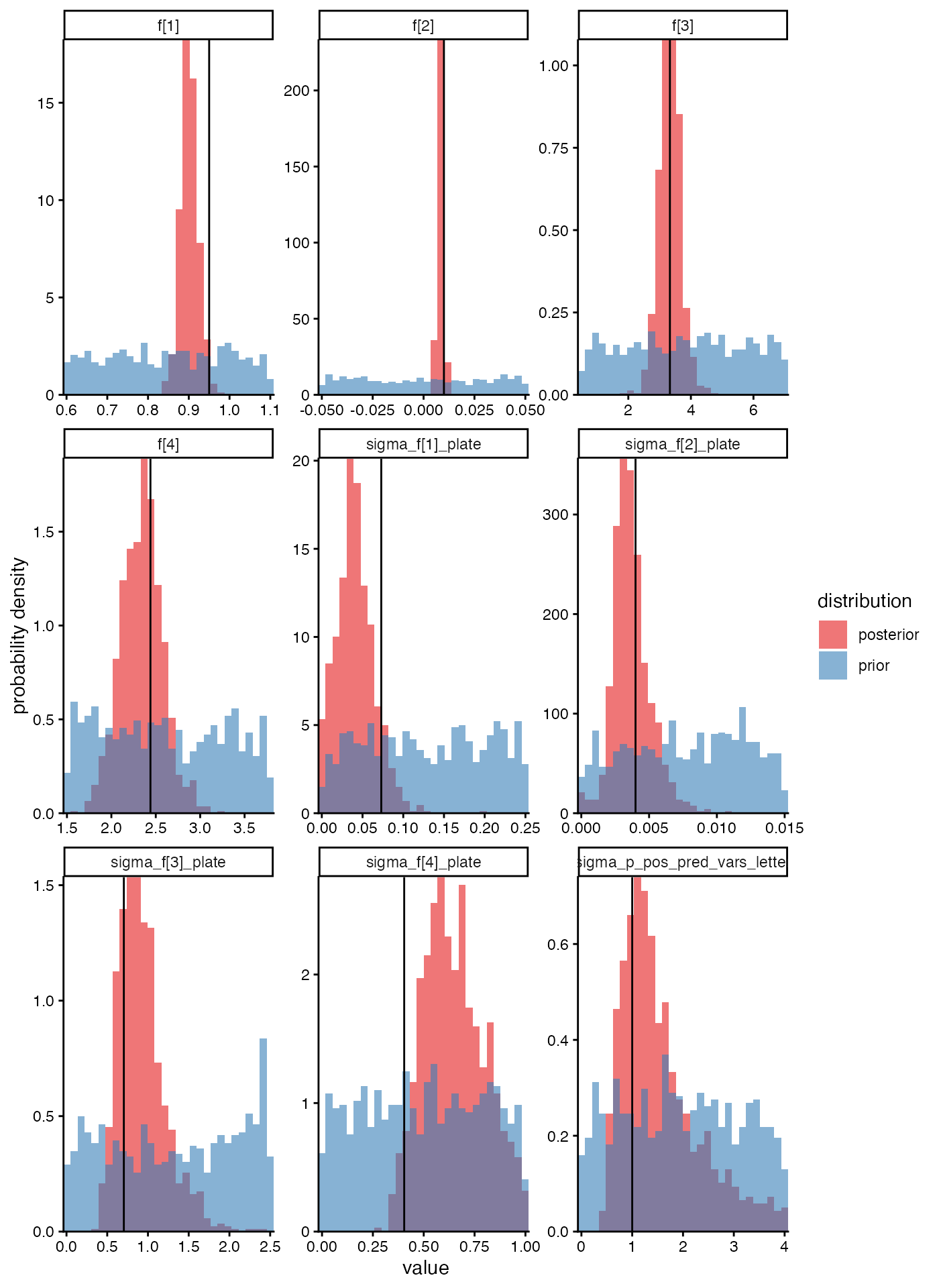

df_posterior has columns named xlog_sam[1], xlog_sam[2] etc. which contain the posterior samples for x (on a log scale) for the sample assigned the integer index 1, and 2, etc. Calculate some quantiles of the posterior for each of the samples, and compare these to the true values which we had in df_sam. The smallest values are slightly overestimated and the largest values are slightly underestimated: this is the phenomenon of shrinkage toward the mean, due to these parameters being random effects.

quantiles <- c(0.025, 0.5, 0.975)
df_sam_x <- df_posterior %>%
  select(starts_with("xlog_sam[")) %>%
  pivot_longer(everything(), names_to = "param") %>%
  extract(param,
          into = "id_sam_int", 
          regex = "xlog_sam\\[([0-9]+)\\]") %>%
  mutate(id_sam_int = as.integer(id_sam_int)) %>%
  group_by(id_sam_int) %>%
  reframe(value = quantile(value, probs = quantiles),
          quantile = quantiles) %>%
  pivot_wider(names_from = quantile, names_prefix = "x_quant_") %>%
  left_join(df_sam %>%
              select(id_sam_int, xlog) %>%
              distinct(),
            by = "id_sam_int")
ggplot(df_sam_x) +
  geom_errorbar(aes(xlog, ymin = x_quant_0.025, ymax = x_quant_0.975)) +
  geom_point(aes(xlog, x_quant_0.5)) +
  geom_abline() +
  labs(x = "True log x",
       y = "Estimated log x")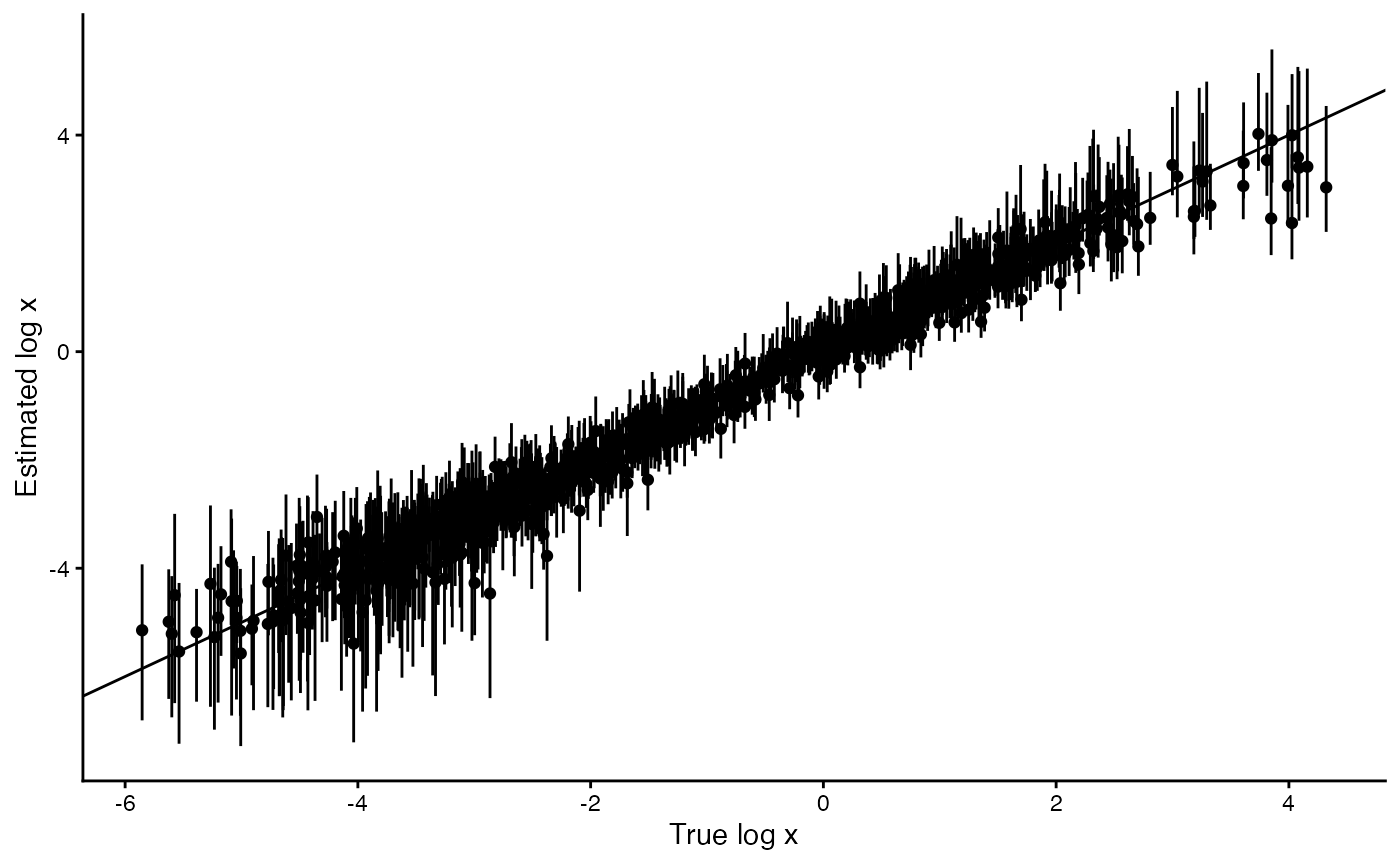

df_posterior has columns named y_sam_sim_unconditional[1], y_sam_sim_unconditional[2] etc. which contain posterior predicted y values for new set of sampled individuals with the same distribution of covariates (i.e. partitioned into the same subpopulations, in this example based on a single covariate letter) as in the dataset analysed. The integer in square brackets indexes the sample replicate as in df_sam$which_sam_rep; we merge df_sam into df_posterior to associated each predicted y value with the appropriate subpopulation. We plot the empirical subpopulation-level distributions of y values, and the posterior predictive distribution of subpopulation-level distributions of y values. We use a log scale for y even though it can be negative, because with our default parameters it’s only rarely negative and a log scale is clearer. We make both a spline density plot and also a histogram (splines are easier to see but the algorithm may make mistakes on fitting a smoothed distribution).

df_y_sim <- df_posterior %>%
  select(starts_with("y_sam_sim_unconditional[")) %>%
  mutate(sample = row_number()) %>%
  pivot_longer(-c("sample"), names_to = "param") %>%
  tidyr::extract(param, 
               into = "which_sam_rep", 
               regex = "y_sam_sim_unconditional\\[([0-9]+)\\]") %>%
  mutate(which_sam_rep = as.integer(which_sam_rep)) %>%
  left_join(df_sam, by = "which_sam_rep") %>%
  mutate(value = log10(value))
ggplot() +
  geom_step(data = df_y_sim,
            aes(x = value,
                y = after_stat(density),
                group = sample),
            stat="bin",
            color="black",
            bins = 60,
            alpha = 0.1) +
  geom_step(data = df_sam,
            aes(x = log10(y), # y,
                y = after_stat(density)),
            stat="bin",
            bins = 60,
            color="blue") +
  coord_cartesian(expand = F) +
  facet_wrap(~letter) +
  labs(x = "log10(OD value)",
       y = "probability density")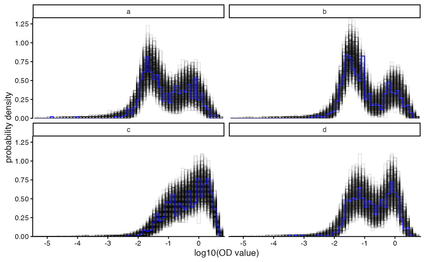

ggplot() +
  geom_density(data = df_y_sim,
               aes(x = value,
                   group = sample),
               color = "black") +
  geom_density(data = df_sam,
            aes(x = log10(y)),
            color="blue") +
  coord_cartesian(expand = F) +
  facet_wrap(~letter) +
  labs(x = "log10(OD value)",
       y = "probability density")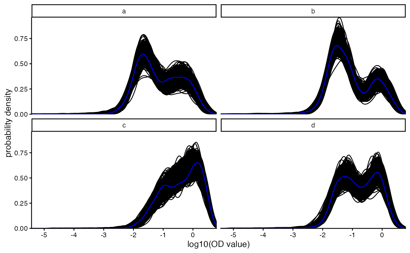

df_posterior has columns named p_sam_is_pos[1], p_sam_is_pos[2] etc. which contain the probability that sample 1, 2 etc. is positive given its observed y values. Calculate the posterior mean for each of these quantities, and then plot the distribution over individuals of these values, stratified by true serostatus. This gives a sense of the model’s accuracy and confidence in estimating serostatus.

df_prob_pos <- df_posterior %>%
  select(starts_with("p_sam_is_pos["))
df_prob_pos <- df_prob_pos[, lapply(.SD, mean)]
df_prob_pos <- df_prob_pos %>%
  pivot_longer(everything(), names_to = "param", values_to = "p_sam_is_pos") %>%
  tidyr::extract(param, 
                 into = "id_sam_int", 
                 regex = "p_sam_is_pos\\[([0-9]+)\\]") %>%
  mutate(id_sam_int = as.integer(id_sam_int)) %>%
  inner_join(df_sam %>% summarise(.by = id_sam_int, pos = unique(pos)), 
             by = "id_sam_int") %>%
    mutate(status = if_else(pos, "pos", "neg")) 

ggplot(df_prob_pos) +
  geom_histogram(aes(x = p_sam_is_pos, y = after_stat(density), fill = status),
                 position = "identity", alpha = 0.6, bins = 30) +
  labs(y = "Number of samples",
       x = "Probability sample is positive") +
  coord_cartesian(expand = FALSE) +
  scale_x_continuous(limits = c(NA, NA))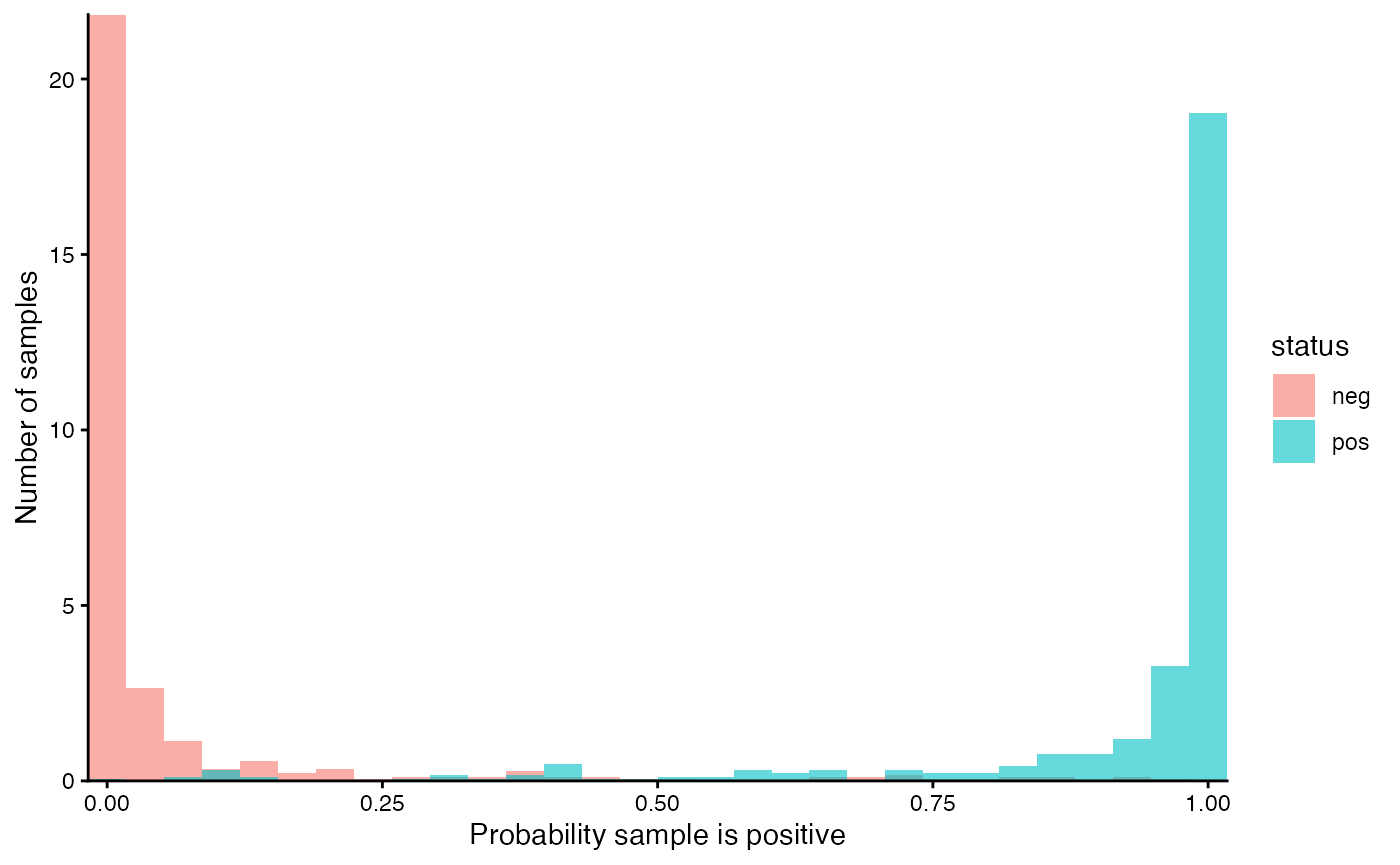

---

1. To sample from the prior we use data_wrangled$stan_input_prior instead of data_wrangled$stan_input_posterior. This samples our parameters using a dataset of the same ‘shape’ (in terms of the definition of regression models with covariates) but no actual samples. This lets us sample the prior for population-level parameters, which are the main thing of interest, forgetting about the individual-level parameters (x values), gaining a lot of speed for big datasets. Note that the fancy sampling algorithm used by Stan (NUTS, a type of Hamiltonian Monte Carlo) is far from the most efficient way of sampling from priors: more efficient would be to sequentially randomly draw a new set of parameters independent of the previous draw, not to use fancy Hamiltonian dynamical equations to make successive draws dependent. Nevertheless we re-use the same Stan code to sample the prior (both in dvsb and in our use of Stan elsewhere) to ensure that the prior we specified in Stan really is what we intended, reducing the potential for silent bugs when sampling from the posterior. The downside is that Stan can have difficulty exploring the geometry of the prior distribution, which will typically be much more disperse than the posterior distribution, so ensure you run enough iterations to get convergence here too.↩︎